

The Ultimate Advisory Role: From Reactive to Predictive
Instead of just talking about cash flow, imagine showing your client visual, data-driven proof of what’s coming. You’re not just telling them about a potential shortfall; you’re presenting a forecast that pinpoints their projected cash balance low point and contrasts it directly with their recent historical high. This shifts the conversation from reactive problem-solving to proactive strategic planning.
This is the pinnacle of strategic treasury advising—moving from analyzing the past to predicting the future. It’s how you build ultimate trust and position yourself to solve a client’s problem before it becomes a crisis. While “forecasting” might sound like the domain of data scientists, modern tools now allow us to perform this analysis right inside the tool we use every day: Microsoft Excel.
In this final post of my series, we will use Python in Excel to efficiently create a time-series forecast of our client’s cash flow, identifying future gaps and creating an undeniable case for a working capital line of credit. We’ll accomplish this using the SARIMA (Seasonal AutoRegressive Integrated Moving Average) method.
The Scenario: Forecasting Cash Gaps for “Global Widgets Inc.”
After analyzing their cash volatility (Part 1) and customer payments (Part 2), Global Widgets is bought in. Their final question is, “What’s next? How do we prepare for the future?” We will use their historical daily cash balance data to build a forecast.
👈 Click to expand
We will use a standard and powerful forecasting method called SARIMA (Seasonal AutoRegressive Integrated Moving Average). It’s excellent at picking up on trends and seasonality in data (like a pre-holiday inventory build-up). The statsmodels Python library makes this advanced technique accessible.
Detailed Steps:
For this analysis, we will use the same daily cash balance data from Part 1. The key is to have a clean, continuous time series.
- Ensure your data is in an Excel Table (
Ctrl+T) namedCashData. - The table must have two columns:
DateandBalance. - Critically, the
Datecolumn must be a continuous daily series. If there are gaps (e.g., weekends, holidays), forecasting models can struggle. We’ll use Python to fill these gaps.
Your starting data table (CashData):
- Activate Python by clicking on the first cell (like D3, outside of the data table), typing =PY and then hitting Tab.
- Paste in this code, which loads the CashData, converts the ‘Date’ column into a proper datetime format, and sets it as the dataframe’s index to prepare it for time-series analysis.
# Load the cash balance data
df = xl("CashData", headers=True)
df['Date'] = pd.to_datetime(df['Date'])
df = df.set_index('Date')- Transforms the data into a consistent daily series (‘D’). It fills in any gaps, such as weekends or holidays, by carrying forward the last known balance (‘ffill’), ensuring a complete daily record for the model.
# Create a complete daily series, filling in missing values
daily_series = df['Balance'].asfreq('D').fillna(method='ffill')- Imports the specific SARIMAX forecasting model from the statsmodels library, which is the statistical engine used for the analysis..
from statsmodels.tsa.statespace.sarimax import SARIMAX- Configures the SARIMA model with parameters for trend (order) and seasonality (seasonal_order) and then trains it on the prepared historical cash balance data.
# Define and train the SARIMA model
model = SARIMAX(daily_series, order=(1, 1, 1), seasonal_order=(1, 1, 1, 7))
fit_model = model.fit(disp=False) # Fit the model quietly- Uses the trained model to generate a 90-day forecast. The results, including the predicted mean values and the upper/lower confidence intervals, are stored in a new dataframe.
# Generate a 90-day forecast
forecast = fit_model.get_forecast(steps=90)
forecast_df = forecast.summary_frame(alpha=0.05) # Include confidence intervals- This is the final, all-in-one script. It executes all previous steps and then uses matplotlib to create the chart. It plots the historical and forecasted data and adds custom annotations and analytical boxes to visually highlight key insights from the forecast.
import pandas as pd
import matplotlib.pyplot as plt
from statsmodels.tsa.statespace.sarimax import SARIMAX
# 1. Load and prepare the data
df = xl("CashData", headers=True)
df['Date'] = pd.to_datetime(df['Date'])
df = df.set_index('Date')
# Create a complete daily series, filling in missing values
daily_series = df['Balance'].asfreq('D').fillna(method='ffill')
# 2. Define and fit the SARIMA model
model = SARIMAX(daily_series, order=(1, 1, 1), seasonal_order=(1, 1, 1, 7))
fit_model = model.fit(disp=False)
# 3. Generate a 90-day forecast
forecast = fit_model.get_forecast(steps=90)
forecast_df = forecast.summary_frame(alpha=0.05)
# --- Plotting Section ---
fig, ax = plt.subplots(figsize=(12, 6))
# 4. Plot historical and forecasted data
recent_data = daily_series['2024-12']
recent_data.plot(ax=ax, label='Historical Balance', color='blue')
forecast_df['mean'].plot(ax=ax, label='Forecasted Balance', color='orange', linestyle='--')
ax.fill_between(forecast_df.index, forecast_df['mean_ci_lower'], forecast_df['mean_ci_upper'], color='k', alpha=0.1)
# --- Annotation Section ---
# 5. Calculate and annotate the VISIBLE historical maximum
historical_max = recent_data.max()
historical_max_date = recent_data.idxmax()
historical_max_date_str = historical_max_date.strftime('%m/%d/%Y')
ax.annotate(
f"Historical Max\n{historical_max_date_str}: ${historical_max:,.0f}",
xy=(historical_max_date, historical_max),
xytext=(historical_max_date + pd.DateOffset(days=20), historical_max + 400000),
arrowprops=dict(facecolor='blue', shrink=0.05, lw=1),
fontsize=9, color='blue', ha='center',
bbox=dict(boxstyle="round,pad=0.3", fc="white", ec="blue", lw=1)
)
# 6. Calculate and annotate the forecasted minimum
forecasted_min = forecast_df['mean'].min()
forecasted_min_date = forecast_df['mean'].idxmin()
forecasted_min_date_str = forecasted_min_date.strftime('%m/%d/%Y')
ax.annotate(
f"Forecasted Min\n{forecasted_min_date_str}: ${forecasted_min:,.0f}",
xy=(forecasted_min_date, forecasted_min),
xytext=(forecasted_min_date - pd.DateOffset(days=20), forecasted_min - 500000),
arrowprops=dict(facecolor='black', shrink=0.05, lw=1),
fontsize=9, color='black', ha='center',
bbox=dict(boxstyle="round,pad=0.3", fc="white", ec="black", lw=1)
)
# 7. Finalize Plot Details
ax.set_title('Global Widgets, Inc: Cash Balance Predictive Analysis')
ax.set_ylabel('Cash Balance (in millions)')
ax.set_xlabel('Date')
ax.legend()
ax.grid(True, linestyle='--', alpha=0.6)
# Set plot date range
start_date = pd.Timestamp('2024-12-01')
end_date = forecast_df.index[-1]
plt.xlim(start_date, end_date)
# Note box in the top-left corner
offset_days = pd.DateOffset(days=3)
y_min, y_max = ax.get_ylim()
ax.text(
x=start_date + offset_days,
y=y_max * .96,
s="Note: Forecast based on last 12 months of data\n"
"Showing December history & full 90-day forecast.",
bbox=dict(facecolor='white', alpha=0.8),
fontsize=9,
verticalalignment='top'
)
# 8. Add cash balance analysis box
balance_travel = historical_max - forecasted_min
# *** ADDED: Calculate the mean of the entire historical series ***
cash_mean = daily_series.mean()
ax.text(
x=pd.Timestamp('2024-12-15'),
y=0,
# *** ADDED: "Cash balance mean" to the text string ***
s=f"Cash balance mean: ${cash_mean:,.0f}\nCash balance travel: ${balance_travel:,.0f}",
bbox=dict(facecolor='whitesmoke', ec='black', boxstyle='round,pad=0.5'),
fontsize=9,
verticalalignment='bottom'
)
plt.show()Deconstructing the Chart & The Python Advantage
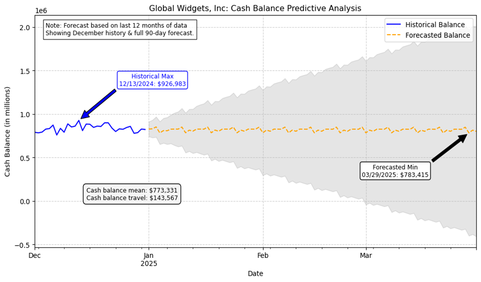
This chart is generated entirely by a Python script within Excel, not manual formatting. It visualizes a 90-day SARIMA forecast based on the client’s last 12 months of daily cash balance data. Key annotations—the Historical Max from December and the Forecasted Min in March—are automatically calculated and placed to highlight the projected “cash balance travel,” or variance.
Interpreting the Forecast
The chart provides a clear, at-a-glance narrative for the client:
- The blue line represents the actual, historical cash balance for December.
- The orange dashed line is the 90-day forecast, showing the most likely path for their cash balance.
- The gray shaded area represents the confidence interval—the range where the balance could plausibly fall.
- The annotated callouts instantly draw attention to the most critical numbers: the highest cash position before the forecast period and the lowest projected point in the near future.
The Advantage: Speed and Flexibility
This is where the Python-driven approach fundamentally outpaces traditional methods.
- It’s Code-Driven, Not Clicks: The entire visual—from the data analysis to the placement of every label and the color of every line—is defined in a single script. This ensures perfect consistency and eliminates tedious manual formatting in Excel’s charting tools.
- It’s Adaptable: Need to analyze a different 12-month period or run the forecast for a different client? Simply change the data source. The script can easily be pointed to a different Excel table, a database, or a CSV file without having to rebuild the analysis from scratch.
- It’s Dynamic: Chart styles, colors, and annotations can be programmatically changed to match a client’s branding or to highlight different analytical scenarios, providing a truly bespoke advisory tool.
The code for this model was developed rapidly by leveraging modern AI tools, including Gemini and Claude models, turning a complex analytical task into a manageable and repeatable process.
The Sales Opportunity:
The forecast makes the need for a solution undeniable and time-sensitive.
By proposing a Working Capital Line of Credit, you’re not just offering a generic credit line; you’re recommending a specific amount tailored to cover the deepest point of the forecasted trough. You can even model the cost of drawing on the line versus the cost of a stock-out or delayed supplier payment. It’s a proactive, consultative sale. The line provides the precise liquidity needed, exactly when the data says it will be needed.
Conclusion: The Evolution of a Treasury Advisor
Across this three-part series, we’ve moved from basic analysis to predictive insight.
- We quantified volatility to sell liquidity solutions.
- We clustered customers to sell receivables solutions.
- We forecasted cash flow to proactively sell financing solutions.
Through the power of AI and by integrating Python’s analytical power into Excel, you demonstrate a modern skillset that goes beyond crunching numbers. You show that you can uncover hidden risks, create data-driven strategies, and act as a true financial partner to your clients. This approach reflects a forward-thinking vision for treasury sales.